
- Services
- Data Analysis services
- Sample Work
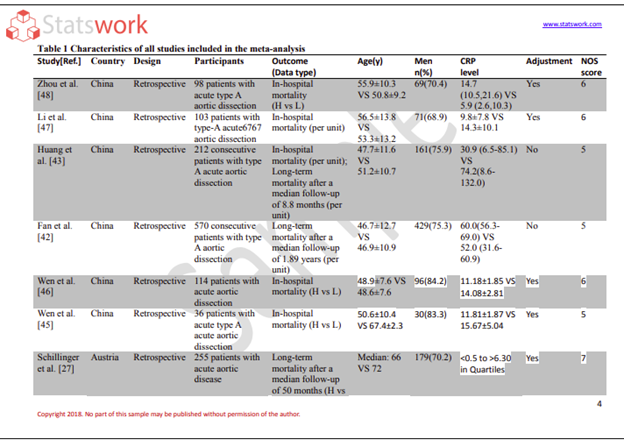
Data Analysis services
- Secondary Qualitative Research Services
- Secondary Quantitative Research Services
- Meta-Analysis Research services
- Sample Work

Meta-Analysis Research Services
- Data Collection Services
- Sample Work
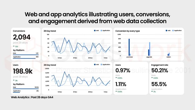
Data Collection Services
- Statistical & Biostatistics services
- Sample Work
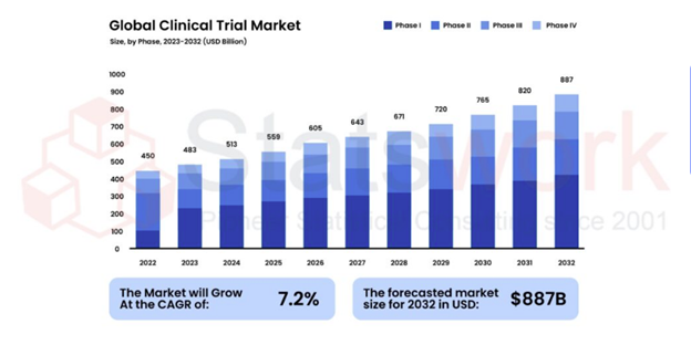
Statistical Programming & Biostatistics services
- Data Management Services
- Sample Work
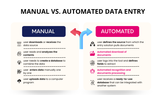
Data Management Services
- Research methodology services
- Sample Work
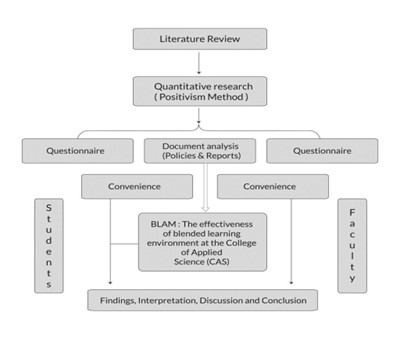
Research methodology services
- Tool Development Services
- Sample Work
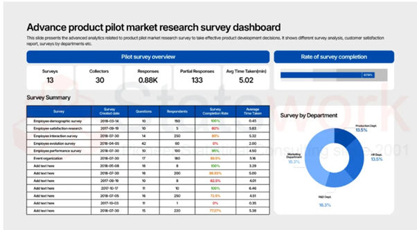
Tool development services
- Statistical Interpretation services
-
Statistical Interpretation services
- Sample Work
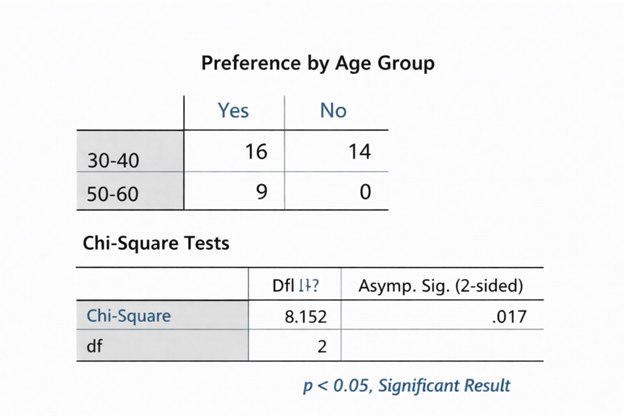
Statistical Interpretation services
-
- Sample Size Calculation Services
-
Sample Size Calculation Services
- Sample Work
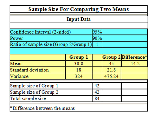
Sample Size Calculation Services
-
- AI & ML Services
-
Artificial Intelligence and Machine Learning Services
- Sample Work
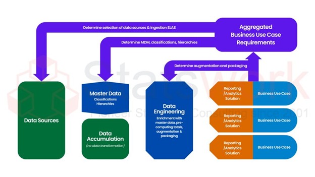
Artificial Intelligence and Machine Learning Services
-
- Meaningful Visualization Services
- Thought Leadership Services
- Report Generation Services
-
Report generation Service
- Sample Work

Report generation Services
-
- Data Analysis services
- Industries
- About Us
- Blog
- Insights
- Contact Us
- Services
- Data Analysis services
- Sample Work
Data Analysis services
- Secondary Qualitative Research Services
- Secondary Quantitative Research Services
- Meta-Analysis Research services
- Sample Work
Meta-Analysis Research Services
- Data Collection Services
- Sample Work
Data Collection Services
- Statistical & Biostatistics services
- Sample Work
Statistical Programming & Biostatistics services
- Data Management Services
- Sample Work
Data Management Services
- Research methodology services
- Sample Work
Research methodology services
- Tool Development Services
- Sample Work
Tool development services
- Statistical Interpretation services
-
Statistical Interpretation services
- Sample Work
Statistical Interpretation services
-
- Sample Size Calculation Services
-
Sample Size Calculation Services
- Sample Work
Sample Size Calculation Services
-
- AI & ML Services
-
Artificial Intelligence and Machine Learning Services
- Sample Work
Artificial Intelligence and Machine Learning Services
-
- Meaningful Visualization Services
- Thought Leadership Services
- Report Generation Services
-
Report generation Service
- Sample Work
Report generation Services
-
- Data Analysis services
- Industries
- About Us
- Blog
- Insights
- Contact Us
How to Interpret Regression Analysis Results: P-values & Coefficients?
Meta Analysis Service
Recommended Reads
Contact us
Summary:
In this blog, I explain the interpretation of regression results based on coefficient, p-value, confidence interval, practical significance, R², and regression assumption. The explanation is given with a regression model with a focus on business and how the result of statistical test could be used for decision making with association versus causation consideration.
Introduction
The budget meeting gets a summary of the regression result in one line: “the effect is significant.” This line is an answer to at least three other questions: the magnitude of the effect, its precision, and whether it calls for action.
In this brief, we illustrate the interpretation of regression analysis in six steps, through one case study of OLS regression analysis [1].
A Worked Example: Does the Loyalty Program Pay Off?
A retailer models monthly spending (US$) for 210 customers with two predictors: loyalty membership (1 = member, 0 = non-member) and app logins per month.
Table 1. Regression of monthly spending (hypothetical data, n = 210)
|
Term |
Coefficient |
Std. error |
t |
p |
95% CI |
|
Intercept |
42.00 |
5.30 |
7.92 |
< .001 |
31.55 to 52.45 |
|
Loyalty membership |
14.20 |
6.10 |
2.33 |
.021 |
2.17 to 26.23 |
|
App logins per month |
3.05 |
0.48 |
6.35 |
< .001 |
2.10 to 4.00 |
|
Term |
Coefficient |
Std. error |
t |
p |
95% CI |
Model fit: R² = .19; adjusted R² = .18; F(2, 207) = 24.3, p < .001; residual standard error = $43.

Step 1: Check Regression Assumptions Before Trusting Any Number
Every number in Table 1 assumes an adequate model, so run diagnostics first (Gelman et al., 2020). Table 2. Diagnostics that most often change conclusions| Assumption | Red flag | What can go wrong? | Solution |
| Linearity | Curved residual plot | Illegitimate estimates | Transformations or nonlinearities |
| Homoscedasticity | Residuals that fan out from centre point | Illegitimate standard errors and p-values | Heteroscedasticity-robust standard errors (Long & Ervin, 2000) |
| Independence | Duplicate rows for each customer/store/region | Overstated significance | Cluster-robust standard errors (Cameron & Miller, 2015) |
| Multicollinearity | Variance inflation factor > 10 | Unstable coefficients | Combine predictors or eliminate redundancies |
| Influential Observations | Large Cook’s Distance | “Some customers determine the effect” | Data check/report results with and without these points |
| Missing values | Output number of cases less than total number of rows [3] | Biased estimates if missing data correlated with outcome | Include missingness information/consider multiple imputations (van Buuren, 2018) |
Step 2: Read Each Regression Coefficient in Its Units
Members pay $14.20 more per month on average relative to non-members that have the same number of logins. Each additional login per month is related to an additional $3.05 spent, while controlling membership status. The constant ($42.00) shows what non-members pay with no login, but this is applicable only when there are actually such customers [4]. Raw coefficient magnitudes should not be compared directly as measures of predictor importance when predictors are measured on different scales. They can, however, be translated into meaningful changes in the outcome for specified contrasts, for example, the estimated $14.20 membership difference is similar in magnitude to the modelled association for roughly 4.7 additional monthly logins). Variable type impacts the interpretation (Gelman et al., 2020): Table 3. How to read a coefficient| Variable or model | How to read the coefficient |
| Continuous predictor | Change per one-unit increase, others held constant |
| Binary or categorical predictor | Difference from the reference group |
| Log-transformed outcome | Each one-unit increase multiplies the outcome by exp(β) (about 100 × β% when β is small) |
| Interaction (X × Z) | X’s effect varies with Z; its own coefficient applies only when Z = 0 |
| Logistic regression | Change in log-odds; exp(β) is an odds ratio, not a change in probability [4] |
Step 3: Read the Confidence Interval Before the P-Value
The p-value, when used correctly, is a valuable statistic (Benjamini et al., 2021). A two-sided p-value of .021 means that, under the null hypothesis and model assumptions, observing a test statistic at least as extreme in absolute value as the observed one would have probability of approximately 2.1%. It is neither 97.9% of the existence of the effect nor an effect size (Wasserstein & Lazar, 2016; Greenland et al., 2016).
The confidence interval gives us useful information for decision making – it shows that the data is compatible with a gap of membership from $2.17 to $26.23 [6].
Multiple screenings increase error rates. When you test 20 predictors independently without any effects at α = .05, there is a 64% chance of obtaining a significant predictor.
All three should be reported: “Membership gap was estimated at $14.20 per month higher spending for members than non-members with similar usage of applications (95% CI $2.17 to $26.23; p = .021).”
Step 4: Separate Statistical from Practical Significance
The American Statistical Association urges not to make business decisions based on p-values crossing the threshold only (Wasserstein & Lazar, 2016).
Assume the cost of the program per member-month was $12. Then, the benchmark would be $12, not zero. The estimate is above the benchmark, but the confidence interval goes as low as $2.17, and the one-tailed p-value of testing against $12 would be .36. Thus, while statistically significant, the outcome is inconclusive about the value of investment in the program even disregarding causality (Step 6).
Sample size may separate the two (Lin et al., 2013). For 60 customers, p would be ≈.22: “not significant,” but not proof of no effect. For 200,000 customers, the tiny difference of $0.70 would get p < .001 (Figure 1) [5].
Figure 1. Estimates and 95% CIs for the membership gap at three sample sizes, against zero and a $12 break even.
Step 5: Interpret R² for What It Measures
An R² of .19 indicates that the independent variables account for only 19% of the variability in expenditure in this data set; it is neither an accuracy percentage nor a percentage of causationR² should not be used by itself to judge whether an individual coefficient estimate is credible. Coefficient uncertainty is assessed through its standard error and confidence interval, while predictive performance should be evaluated separately using appropriate out-of-sample metrics when prediction is the goal. (.18).
Step 6: Use Causal Language Only When the Design Supports It
In observational data, high spenders could have a higher probability of opting in (selection bias), and customers could have a higher number of logins since they make more purchases (reverse causality). Controlling for logins would also be misleading as if the program leads to logins, then controlling for logins means that one does not capture all effects of the program (Gelman et al., 2020) [6].
Causal interpretation requires an identification strategy and assumptions appropriate to the research design, for example randomization, difference-in-differences, regression discontinuity, instrumental variables or other defensible causal-inference approaches. Before any design evidence is available, one should write “members spend more” instead of “the program increases spending.”
From Regression Output to a Defensible Business Decision
The time taken to read table 1 is just a few minutes. Whether to conclude that the table supports justification of budgeting, pricing, or customer recommendations is based on how the table is designed, diagnosed and based on the decision-making criteria.
The services of Statswork on multiple regression analysis involve those aspects. The statisticians at Statswork ensure that the model fits your business problem, does the above diagnoses and checks the effects of the regression against your break-even point and not zero.
Send Statswork your regression output or dataset for a statistician’s review before it reaches a board paper or client report.
Frequently Asked Questions (FAQs)
The outcome is estimated to fall as the predictor rises, other predictors held constant. The sign shows direction, not importance; if it flips when a correlated predictor is added, suspect multicollinearity or confounding.
No. The data lack strong evidence against a zero effect. A CI spanning both zero and practically important values means the result is inconclusive, often because the sample is too small (low statistical power).
No universal threshold exists. A modest R² can suit a model built to estimate a relationship; judge forecasting models on out-of-sample prediction error.
References:
- Benjamini, Y., De Veaux, R. D., Efron, B., Evans, S., Glickman, M., Graubard, B. I., He, X., Meng, X.-L., Reid, N., Stigler, S. M., Vardeman, S. B., Wikle, C. K., Wright, T., Young, L. J., & Kafadar, K. (2021). The ASA president’s task force statement on statistical significance and replicability. The Annals of Applied Statistics, 15(3), 1084–1085. https://doi.org/10.1214/21-AOAS1501
- Cameron, A. C., & Miller, D. L. (2015). A practitioner’s guide to cluster-robust inference. Journal of Human Resources, 50(2), 317–372. https://doi.org/10.3368/jhr.50.2.317
- Gelman, A., Hill, J., & Vehtari, A. (2020). Regression and other stories. Cambridge University Press. https://doi.org/10.1017/9781139161879
- Greenland, S., Senn, S. J., Rothman, K. J., Carlin, J. B., Poole, C., Goodman, S. N., & Altman, D. G. (2016). Statistical tests, P values, confidence intervals, and power: A guide to misinterpretations. European Journal of Epidemiology, 31(4), 337–350. https://doi.org/10.1007/s10654-016-0149-3
- Lin, M., Lucas, H. C., Jr., & Shmueli, G. (2013). Research commentary—Too big to fail: Large samples and the p-value problem. Information Systems Research, 24(4), 906–917. https://doi.org/10.1287/isre.2013.0480
- Long, J. S., & Ervin, L. H. (2000). Using heteroscedasticity consistent standard errors in the linear regression model. The American Statistician, 54(3), 217–224. https://doi.org/10.1080/00031305.2000.10474549